Before we begin, you may bring a cup of coffee that can help us through the paper.
Overview
Paper link: https://arxiv.org/pdf/2012.12160.pdf
Authors: Justin Liang, Namdar Homayounfar, Wei-Chiu Ma, Shenlong Wang, Raquel Urtasun
In this paper, the authors propose a neural network that extracts the drivable road boundary from LiDAR and camera image input.
Extraction of drivable road boundary is important for self-driving cars. In this paper, the authors propose a convolutional recurrent network that extracts the road boundary from LiDAR and camera input.
Preliminary
If you are not familiar with the followings, check out the blog posts.
Keywords
CNN, HD map, Curb detection, LiDAR, Distance transform, FPN, Skip connections, Dilated convolutional layers, Instance normalization, STN
Problem definition
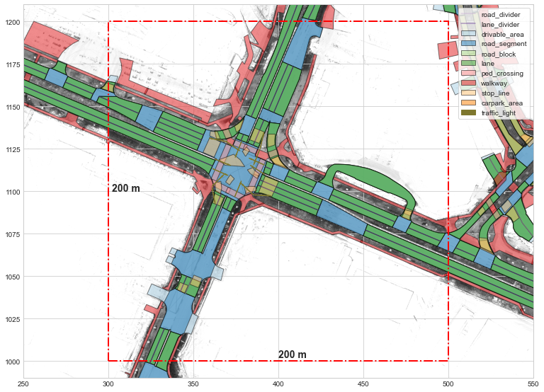
As we have discussed about HD maps (High Definition maps) in the post, one of the limitations of HD map is that its annotation is awfully laborious. Hence, there have been numerous efforts to automate the map construction process.
In this paper, the authors focus on the extraction of the drivable area from LiDAR and camera input, employing the convolutional neural networks (CNN) and convolutional recurrent network (CRNN).
What are the inputs?
3D point cloud data from LiDAR and 2D images from RGB camera are the available raw sensor modalities. However, they can not be directly consumed by the model, since the nature of the data from two sensors are completely different. How can you directly combine the 3D unordered points from LiDAR and 2D 3-channel pixels from camera together?
Thus, the authors create bird-eye view (BEV) representations of the sensor readings and use them as the input to the system. In other words, the lidar point cloud data is projected onto the $x$-$y$ plane, then translated into an image.Though not stated explicitely in the paper, a 3D to 2D projection, or “flattening” of the point cloud data can be easily done by removing the z-axis — something like, pts_2d = pts_3d[:, :2].
At this point, some might argue: “Wait, how can you just remove a dimension? Doesn’t that kinda… lose some information?” Well, that’s completely correct. Simply removing the last column (which is z-coordinates) will lose some data. Therefore, in order to keep our precious 3D information, one or more additional channels are usually added to the input tensor of the LiDAR so that the “height” information can be preserved. This post discusses about various ways of achieving the goal.
The authors stipluated that they added the gradient of the height value as an extra channel:
We also input as an extra channel the gradient of the LiDAR’s height value. This input channel is very informative since the drivable and non-drivable regions of the road in a city are mostly flat surfaces at different heights that are separated by a curb.
Long story short, the input is a 5-dimensional image that is generated by the BEV representation of the LiDAR point cloud and the top-view image. The point cloud data from LiDAR is first projected onto the grid in the $x$-$y$ plane, and to each pixel the intensity and the gradient of the height value are assigned. This is then concatenated with the corresponding RGB image, resulting in a 5-dimensional input image. Mathematically speaking, each input tensor is
\[I \in \mathbb{R}^{5 \times H \times W}\]where $H$ and $W$ is the height and the width of the input image.
What is the desired output?
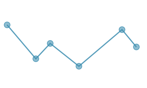
For a given input $I \in \mathbb{R}^{5 \times H \times W}$, the desired output is a list of vectorized road boundary. Each road boundary is a polyline, which basically is a ordered list of $\left(x, y\right)$ coordinates.
Mathematically speaking, the output $O$ can be expressed as
or, in a more computer science format,
output = [[(x0_0, y0_0), (x0_1, y0_1), ...],
          [(x1_0, y1_0), (x1_1, y1_1), ...],
          ...
          [(xi_0, yi_0), (xi_1, yi_1), ...],
          ...
          [(xn_0, yn_0), (xn_1, yn_1), ...]]
Notice that the output is a list of polylines. A polyline is an ordered set of point, which when connected sequentially, produces a line of interest.
So, what’s the plan from input to output?
Remember that the input was a 5-dimensional image, but the desired output is a set of polylines. In other words, we want a set of point coordinates as output. However, a CNN is designed for the images, since it applies the weights and biases to the pixels. What should we do?
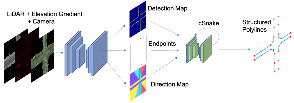
Here’s the plan. As an intermediate step, we will train the model that outputs one or more feature maps or visual cues (since the feature maps are “images”), and we are going to apply another algorithm that generates a set of point coordinates from the feature maps. The authors refer to the module that generates a set of polyline from the feature maps as “cSnake”.
Easy, right? But, one question still remains. What kind of feature map are we looking for? In other words, what kind of images do we expect our model to translate the input image into?
It would be great if the feature maps have properties that are useful for the extraction of the polylines. As to achieve this goal, the authors suggest three feature maps: detection map, direction map, and endpoint map, which are denoted as $S$, $D$, and $E$, respectively.
Let us take a look at each of the feature maps.
Detection map: how much more should I go?
First, a detection map. Authors define a detection map to be an inverse truncated distance transform image.
“A… what?”
If you are stuttering, don’t worry. Let’s dissect it one by one.
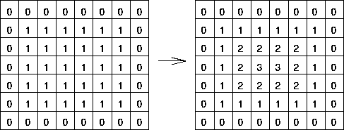
Let us first briefly review what distance transform is. A distance transform, or a distance map, is a map where each pixel represents the distance to the nearest boundary pixel. Take a look at the figure below.
If you are still confused and want a bit more of distance transform, this post will be helpful.
Suppose our model did a good job on predicting the inverse truncated distance transform image. Then we can generate the polyline by finding the points that maximizes the detection map values.
But, why would we want to invert the values of the detection map? The reason will become clear when we move on to the direction map.
Direction map: where should I go from here?
Let’s say we have successfully generated a detection map. It means for each pixel on the BEV image, we know how far we are from the nearest curb. However, that is not what we want. At the end of the day, we want to find the exact location of the curb in a form of polyline. Thus, we need an information of where to move in order to find a curb.
Intuitively, we can take a partial derivative of the detection map with respect to each direction — or, take the gradient ($\nabla$) of the detection map — in order to obtain the direction map.
Note that the result of gradient operation is a vector; thus, the authors stipulate that the direction map is a vector field, i.e.,
\[D \in \mathbb{R}^{2 \times H \times W}\]How do we take the gradient of an image? We can implement a partial derivative operation, but we already have a splendid kernel that does the task that we’re after, namely, the Sobel filter. The Sobel filter is a special type of a filter used in CNN, which is particularly used for the edge detection. It is a discrete differentiation operator, which computes an approximation of the gradient of the pixel value of the image. The authors state that they have used the Sobel derivative to obtain the direction map.
We obtain the ground truth by taking the Sobel derivative of the road boundaries’ distance transform image followed by a normalization step.
Aha, now we understand why the authors used the inverse distance transform. If we take the sobel derivative of the inverse distance transform, the direction would be naturally pointing towards the nearest curb, since the direction of the gradient vector is always heading towards where the value increases the most rapidly.
Quick tip for Physics students
If you are a Physics student and are familiar with the field theory, you can think of a distance map as a potential field and a direction map as a force field.
Also, Bear in mind that the detection map is the inverse distance map, so we don’t have to account for the negative sign in front of the following relationship:
\[\vec{F} = - \vec{\nabla} \cdot U\]Endpoint map: where should the curb begin?
Lastly, we need a point from which we can begin constructing the polyline. The authors propose to use a heatmap that encodes the probability of each pixel of being an endpoint. In other words, each pixel of the endpoints heatmap stores a value between 0 and 1, which tells the probability of the pixel of being an endpoint; if the point can function as an endpoint, it will have a value close to 1; if not, it will have a value close to 0.
Also note that the endpoint heatmap has a dimesionality of
\[E \in \mathbb{R}^{1 \times H \times W}\]Why use detection map and direction map, if we can use heatmap for all?
At this point, a question might arise in reader’s mind.
“If we can generate a heatmap/binary map that encodes the probabiliry of each point belonging to the curb, shouldn’t that to the work? We might just have to connect the points where the probability is higher than the threshold.”
Well, the reason we want to output the detection map and the direction map is that, they are dense maps and thus can encode more information about the locations of the road boundaries. According to the authors,
In contrast to predicting binary outputs at the road boundary pixels which are very sparse, the truncated inverse distance transforms encodes more information about the locations of the road boundaries.
There are many cases in reality where the location of the curb should be inferred from the context. For example, in most cases, there will be a huge change in height at the curbsides. However, this might not be true for some cases, such as at the crosswalks, roll curbs, or curb ramps. The curb might simply be under construction or is partially destroyed. For such cases, the deep learning model should be able to think from the context, which a binary map or a heatmap cannot provide.
Suppose you are provided with a binary map, or a heatmap that encodes the location of the curbside. Your task is to find a polyline of the curbs. You might first connect the obvious points, i.e., where the binary map is 1 or where the heatmap is close to 1.
But, what next? The distribution of the 1s is likely to be pretty noisy. Here is where the contextual reasoning comes into play. You can do something like:
“Well, since I have a chunk of points from which I deduced one line segment here, and another over there, and they kinda look like they belong to the same curb, lemme connect these two to continue my polyline.”
This is exactly what we expect our model would be doing. Or, at least similar to what we are expecting from the model. The kinda look like they belong to the same curb part is taken care by the detection map and direction map, since the contextual information that each pixel of the feature map is holding can tell if the line segment here and there belong to the same curb.
Okay, it’s time to get real. Let us take a look at the network that is capable of performing the tasks mentioned above.
Network architecture
The authors used a encoder-decoder architecture similar to FPN. A FPN, or a Feature Pyramid Networks, is a network that is designed to carry out the object detection task in various scale.
An FPN consists of two parts: a bottom-up pathway and a top-down pathway. At each corresponding stage in bottom-up and top-down pathways, the lateral connection combines the low-resolution, semantically strong features from the top-down pathway with high-resolution, semantically weak features from the bottom-up pathway. Take a look at the following post for more information about FPN.
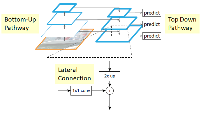
The authors mention that they chose the FPN-like network because of its efficiency and its ability to keep spatial information. Remember that the skip connections between the encoder and decoder can recover the lost spatial information.
Encoder
The encoder part of the network consists of several encoder blocks, each of which corresponds to the “stage” from FPN. Each encoder block contains two residual blocks, and each residual block contains three dilated convolutional layers.
The dilated convolutional layers is useful for its ability in increasing the receptive field without losing much spatial dimension. More of the dilated CNN can be found from the following post.
Decoder
The decoder part consists of the same number of decoder blocks as the encoder blocks. Each decoder block contains four convolutional layers. To the end of each decoder block is attached a nearest neighbor upsampling of 2x.
For both the encoder and the decoder part, prior to each convolutional layer, the instance normalization followed by a ReLU activation layer is attached.
Output branches
The network has three output branches, corresponding to the distance transform, endpoints heatmap, and direction map, accordingly. The feature maps generated from the output branches all have the same spatiala dimension as the input imate $I$.
Learning
For the learning of the feature maps, the following loss is used.
\[l\left(S, E, D\right) = l_{det}\left(S\right) + \lambda_1 l_{end} \left(E\right) + \lambda_2 l_{dir} \left(D\right)\]The regression loss is used for the distance transform $S$ and the endpoint heatmap $E$, and the cosine similarity loss is used for the direction map $D$.
Also, the loss weighting parameters $\lambda_1$ and $\lambda_2$ are experimentally determined to be 10. This is to balance the magnitude of each loss components so that the learning process won’t be biased.
Now that we have all the key feature maps that can be helpful for the generation of the road boundary, let us take a look at the road boundry extraction module, or cSnake, as the authors refer to as.
Road boundary extraction module
Making use of the feature maps predicted by the FPN-like encoder-decoder network, we are now ready to extract the road boundary. Remember that what we want in the end is a set of polylines, where each polyline is a sequence of points. The author proposes that this can be done by iteratively outputting the vertices of a polyline corresponding to a road boundary.
Let me elaborate on this a bit more. First, we begin from finding the initial vertex $x_0$ of the road boundary by analyzing the endpoint heatmap $E$. It can be done by computing the local maxima of $E$.
Next, we compute the direction vector $v_0$ at point $x_0$. The direction vector is where the road boundary will be “propagating” forward, and can be found through the following steps. First, we pick a pixel from the direction map $D$ which is closest to the initial vertex $x_0$. The direction vector from $D$ at this pixel should be “pointing towards” the road boundary, either from left to right or from right to left. In either cases, we can obtain $v_0$ by rotating this vector by 90 degrees, pointing away from the “cropped image boundary”.
Now, using the vertex $x_0$ and the direction vector $v_0$, a rotated ROI can be cropped, using a Spatial Transform Network. The rotated ROI is cropped from the concatenated image of the detection map $S$ and the direction map $D$. This rotated ROI is fed into a CNN, which computes the next vertes $x_1$. The detailed structure of the CNN will be illustrated below.
More on Spatial Transform Network (STN) can be found from the following post.
This is a single step for locating $x_1$, the point on the road boundary that follows the initial vertex $x_0$. From here, the processes mentioned above can be repetitively applied in order to continue the polyline; i.e., compute $v_1$ from the direction map $D$, then apply a STN to extract the ROI, and input the rotated ROI into a CNN to locate the next vertex, $x_2$.
Network Architecture of the extraction module
The road boundary extraction module described above requires an additional CNN that takes in a rotated ROI that is cropped from the concatenation of $S$ and $D$, and predicts the next vertex. The network architecture of the CNN is as follows.
The CNN has an architecture that is identical to the encoder-decoder backbone that is used for the prediction of the feature maps, except for that it has one less convolutional layer in both the encoder and decoder blocks.
The output of the CNN is a score map, whose argmax can be used to obtain the next vertex for cropping.
Learning
For the learning of the CNN used as part of the extraction module, the following loss is used.
\[L \left(P,Q\right) = \sum_{i}\min_{q \in Q} ||p_i - q||_2 + \sum_{i}\min_{p \in P} ||p - q_j||_2\]Here, $P$ is a predicted polyline and $Q$ is a ground truth road boundary, and $p$ and $q$ are the rasterized edge pixels of $P$ and $Q$ respectively.
| Be careful, we are not looking at the vectorized vertices, i.e., something like $p_i = \left(x_i, y_i\right)$. We are interested in the pixel values, where we take a look at each and every pixel values of the image, i.e., $ \{p_i | p_i \in \mathbb{R}^{H \times W} \} $. |
Notice that the loss above is a L-2 Chamfer Distance between the polyline and the ground truth boundary. A distance map $D$ can be helpful for this computation. Why? Suppose we want to compute the term
\[\min_{q \in Q}||p_i - q||_2\]for some pixel $p_i \in P$. Then, all we have to do is simply take a look at the value from the distance map $D$ at the corresponding pixel value, since it already contains the information of the distance to the nearest boundary, which is exactly what we’re after.
More on distance metrics such as Chamfer Distance and Wasserstein Distance can be found from the following post.
Evaluation
The authors provide the experimental evaluation result in the paper.
Dataset
The dataset that is used for the training of the model consist of BEV projected LiDAR and camera images, which amounts to 4750km of driving, 50km$^2$ of area.
The LiDAR dataset contains approximately 540 billion points in total. Also, the images has the dimension of 1927px ($\pm$893) $\times$ 2162px($\pm$712), with 4cm/px resolution.
The LiDAR point clouds and camera images are tiled and splitted into 2500, 1000, 1250 train/val/test sets.
Metrics
The metrics used for the evaluation of the performance of the model is as follows.
Precision and Recall
The definition of precision and recall is detailed in the following post.
The precision and recall metrics are used to tell if the points on the predicted poylines are within the threshold of the ground truth polyline.
Connectivity
The authors proposes the following metric to evaluate how well the predicted polylines are “connected”.
\[\text{Connectivity} = \frac{1}{M}\]Here, $M$ is the number of predicted polylines that is assigned to a single ground truth polyline. For example, if for a ground truth polyline the model predicts two polylines, the connectivity is $\frac{1}{M}=\frac{1}{2}=0.5$.
The connectivity is at its maximum of $1$ when the model successfully propagates through the ground truth polyline from beginning to end, resulting in $M=1$.
$M$ is assumed to be a positive integer value; i.e., we ignore the case where the model fails to assign any prediction to the ground truth polyline.
Evaluation result
Below is a evaluation result. The authors compared the distance transform (DT) baseline with their model.

Inference
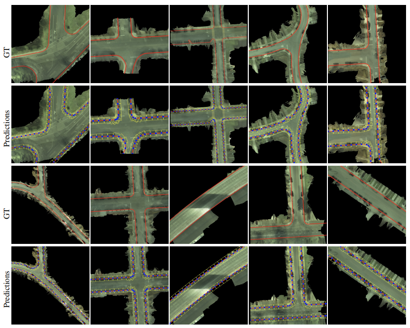
Below are some inference results.
Conclusion
The road boundary extraction algorithm proposed by the paper could successfully extract the road boundary from the given LiDAR point cloud and camera imagery data. However, there were several limitations.
- Endpoint heatmap is not a robust method to account for cases where the road boundary is not clear, vanishes, or merges/splitted. These cases might result in the situation where it might not be possible to begin/conclude the cSnake module.
- The paper does not explain much about the vertical hindrance; i.e., the possibility of street trees/lamps blocking the BEV LiDAR/camera data.
Great, we made it to the end of the paper. If you find this post useful, or have any questions/comments, please leave a comment.

Leave a comment