Project Team member: Youngwoong Cho, Rose Gebhardt, Frederick Rapp, Marina Akopyan

Introduction

One of the most known datasets in architecture is the Neufert Architects dataset. This is a collection of objects and spaces categorized by function and dimension. Furniture pieces are specified with dimensions that are required to meet a comfortable living style. These various dimensions and uses of furniture are drawn in detail and obsession in this book. Using this as a starting point for data findings, we wanted to begin to challenge the specificity of furniture and its uses.

This project uses furniture as a basis for cross contamination of function. Using datasets of different furniture types, the latent space will be created using the deep autoencoder. From the created latent space, vector operations between different types of furniture will be implemented to create a new type. A lamp and a chair are two distinct pieces often with similar elements, but when merged together they could begin to generate new ways of living at home. The outcome generated morphs between two types of furniture and resulted in an abstraction and essential form of the furniture that is seen.

Process

Model design

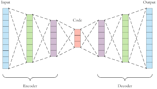
The neural network architecture used in the project is a deep autoencoder.

Deep autoencoder consists of an encoder and a decoder connected by a bottleneck layer. Both the encoder and the decoder consist of several fully connected layers. The difference is that the encoder “compresses” the complexity or dimensionality of the data by passing the data through the layers of lower dimensions, whereas the decoder “reconstructs” the data by passing the data through the sequence of layers that increases in dimensions.

Our model has an encoder with three fully connected layers, whose output dimensions are 128, 64, and 32, respectively. Also, our model has a decoder with three fully connected layers, whose output dimensions are 64, 128, and 3 times the image size squared (3$\times$img_size$^2$), with the image size (img_size) being the number of pixels of the height and width of the input image.

The layer between the encoder and the decoder is called the bottleneck layer, and the number of the dimension of the bottleneck is called encoding dimension. The smaller the encoding dimensions, the more the data is compressed. Our model has the encoding dimension of 32.

Dataset

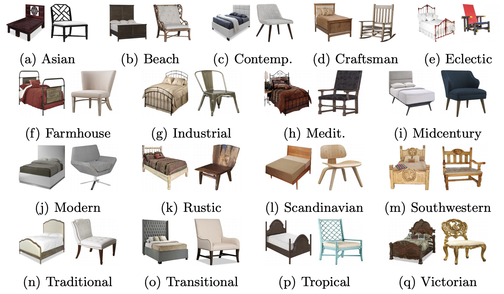
We used various images of the furnitures that are available from Bonn Furniture Style Dataset The dataset contains 90,298 images from 6 categories of furniture across 17 different styles.

Result

Latent space interpolation

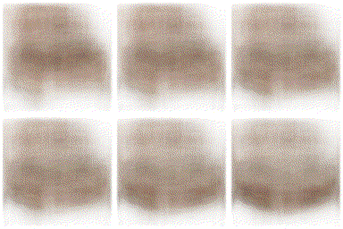
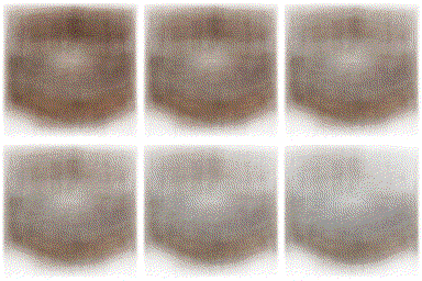
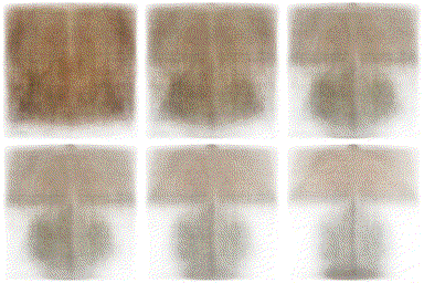
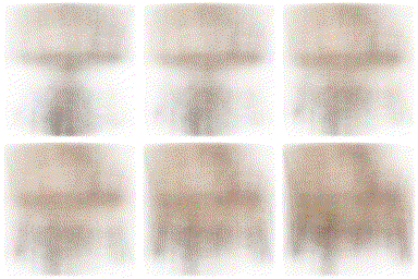
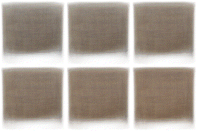
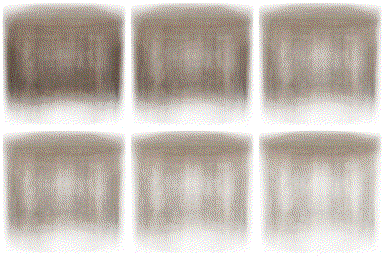
Below is the latent space interpolation among different types of furnitures.

t-SNE clustering

We then visualized the latent space created by the model. Since 32-dimensional vectors cannot be visualized directly, we used t-SNE algorithm to visualize the vectors in 2-D space. The combinations of the furniture types that showed more distinct transition during the latent space interpolation are expected to have more distinct clustering in the latent space distribution. Following figures show the resulting latent space visualizations. Each datapoint is color-coded so that different types of furniture are colored differently.

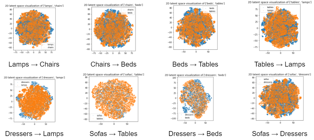
The resulting latent space did not exhibit a clear clustering. This can be attributed to several reasons. First, the number of iterations was not enough for t-SNE algorithm to fully perform the clustering. Also, changing the hyperparameters such as perplexity will help the clustering from being trapped in the local equilibrium where the cluster is not well formed.

The code of the project can be found from the following Github link.